Aloha Norden: Population Sizes and Chaotic Music

Let's think about a very simple model of population growth. Say at any given time the popualtion is at some fraction of the total possible, like 10%, 50%, or 90%. We can represent this as 0.1, 0.5, or 0.9 respectively. The current population can grow at a certain rate, r. Let's say the current population fraction is x. We can multiply r and x to get the size it has grown into in the next generation. Let's call the next generation x'. So we get a simple formula, x' = r x. If r is 1 the population stays the same size (on average each individual produces only one descendant for the next generation). If it is greater than one the population grows in size.

OK, the population can not grow past 100% of its total carrying capacity. So if it gets too large and uses up all the resources (food, shelter, etc.) the population will shrink (die off) by some amount. To take this into account we can multiply (1 - x) --the distance the population is from the maximum size--in our model. So now we have x' = r x (1- x ). This is a very simple formula to model population growth, but it has some very interesting properties.

Now, if the growth rate is only 1, r = 1, the population declines in size because some resources are used up. With a growth rate of two the population approaches an equilibrium at 50% of its maximum size; it doubles each generation but half of the resources are used up, cutting it back in half again. What happens with an even higher growth rate, 2.8. (An average of almost three offspring per adult.)

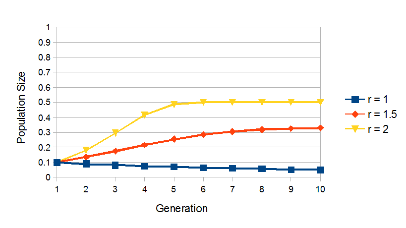
Now the population overshoots the equilibrium a bit. When the population size is low there are plenty of resources and a large number of offspring, but the large number of offspring means even more resources are used up in the next generation and so there are less surviving offspring. The population size oscillates for a few generations until settling down on an equilibrium value. (This is called a dampened oscillation.) What happens if the growth rate is even larger?

With an average of 3.3 offspring (6.6 per couple) the population approaches a stable oscillation. It uses up too many resources, crashes, rebounds, uses up resources, crashes, rebounds, .... At equilibrium it alternates between two sizes, like over-correcting while steering a car or bicycle.

At an even higher growth rate, r = 3.55, another shift in behavior occurs. The population is still oscillating in size, but it takes four generations to return to the same point. It is as if the population overgrows a lot, crashes by a huge amount, grows less from the lower number, crashes less from the lower peak, overgrows a lot, ... Importantly, though, trajectories starting from slightly different values still converge to the same cycles (in the figure above one population starts at x = 0.1, blue, and the other is x = 0.15, orange, in generation 1).

Some organisms can have 100s of offspring. What happens if we raise the growth rate even more?

After a certain point we encounter chaotic behavior. The changes in size do not follow an obvious pattern and small differences in starting values result in widely different, divergent, trajectories a few generations later.

However, it is important to keep in mind that these changes are not random and are solely determined by the simple equation, x' = r x (1- x ). If we plot x' versus x, from generations 5 to 40, we see that the points jump back and fourth but fall along a simple curve and start to fill in something like a inverted parabola shape.

If we plot the equilibrium point(s) that are approached by x (the population size) over a range of r (the per generation growth rate) we get this type of diagram.

So, as in the examples I illustrated above for r = 2.7 a single equilibrium value of x is approached. For an r = 3.2 the system tends to oscillate between two points. At about r = 3.5 it moves between four points. Then briefly as r increases there is an 8 point oscillation (and if you look closely at the r = 3.55 example above you can see it is actually visiting 8 points rather than 4 I said above) and after this point it quickly becomes so complex that a wide range of points are visited and we get chaotic behavior. However, you can also see gaps in the chaos where the system suddenly settles down and oscillates between only a few points before becoming chaotic again. This is the classic bifurcation diagram of the logistic map in chaos theory.

So this is a complex system but there is a relationship between nearby points in time, kind of like the notes in music. (A search online shows I am not the only one to think about this, here is an example). I've been curious about this and finally got around to converting x values from 0-1 to a MIDI file with notes in an octave scale. The MIDI can then be converted to WAV (http://www.hamienet.com/midi2mp3) and sheet music (http://www.8notes.com/) formats online.

The first example moves along the logistic map. I slowly increase r each generation and let x (sound pitch) follow along. You can hear the notes growing, then oscillating in a simple pattern, then more complex, then chaos, settling down into a simple pattern again, then back to chaos. I'll put the logistic map here again to follow along. As the music plays follow the curve from left to right.

Yes, I know it is a bit maddening to listen to (V made that clear to me when I was tweaking the sound and playing it over and over at home earlier), but it also has some interesting points and I dare say is not the worst music ever made (certainly not the worst I have made).

Next is an example with two notes generated with two different fixed values of r, 3.6 for the lower note and 3.9 for the higher one. It sounds demented but there are some textures that fade in and out near the middle of the recording.